Pulse shaping and matched filtering

A pulse $p(t)$, with time measured in symbol periods, satisfies the Nyquist criterion if $p(0) = 1$ and $p(n) = 0$ for every nonzero integer $n$. The raised-cosine pulse is a Nyquist pulse. A common choice is to use its square root at the transmitter, and the matched filter at the receiver, whose taps are those of the transmitter reversed in time (the same, since the pulse is even). The autocorrelation of the root-raised-cosine pulse is the raised-cosine pulse, so the output of the matched filter passes through the symbols at the symbol instants. For more details, see PS08, Sec. 9.2–1.

>>> import numpy as np
>>> import komm

>>> constellation = komm.PAMConstellation(4)
>>> symbols = constellation.indices_to_symbols([3, 2, 1, 2, 0, 1, 2, 0, 3, 2])
>>> symbols
array([ 3.,  1., -1.,  1., -3., -1.,  1., -3.,  3.,  1.])

>>> pulse = komm.RaisedCosinePulse(rolloff=0.25).root()
>>> sps = 20
>>> taps = pulse.taps(samples_per_symbol=sps, span=(-16, 16))
>>> upsampled = komm.sampling_rate_expand(symbols, factor=sps)
>>> signal = np.convolve(upsampled, taps)
>>> filtered = np.convolve(signal, np.flip(taps)) / sps

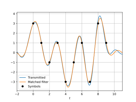
The first convolution places a pulse at each symbol; the second one approximates the integral of the matched filter, hence the division by the number of samples per symbol. Each filter delays the signal by $16$ symbols, half the span of its taps. At the symbol instants, the output of the matched filter gives back the symbols, while the transmitted signal does not, since the root-raised-cosine pulse is not a Nyquist pulse:

>>> komm.sampling_rate_compress(filtered, factor=sps)[32:42].round(2)
array([ 3.,  1., -1.,  1., -3., -1.,  1., -3.,  3.,  1.])
>>> komm.sampling_rate_compress(signal, factor=sps)[16:26].round(2)
array([ 2.96,  1.09, -1.11,  1.09, -3.01, -1.1 ,  1.22, -3.31,  3.34,  0.68])

To plot the signals, with Matplotlib:

import matplotlib.pyplot as plt

fig, ax = plt.subplots()
ax.plot(np.arange(signal.size) / sps - 16, signal, label="Transmitted")
ax.plot(np.arange(filtered.size) / sps - 32, filtered, label="Matched filter")
ax.plot(symbols, "ko", label="Symbols")
ax.set(xlabel="$t$", xlim=(-2, 11))
ax.grid()
ax.legend()
plt.show()

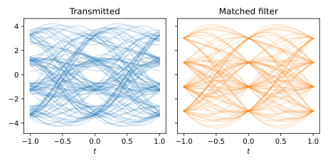
The eye diagram shows the same for many random symbols, by overlaying segments of the signal that span two symbol periods, centered at the symbol instants. With mode="valid", each convolution keeps only the samples not affected by the edges of its input, and starts at a symbol instant. Rounded to two decimal places, the samples of the output of the matched filter take only the values of the constellation:

>>> rng = np.random.default_rng(seed=42)
>>> komm.global_rng.set(rng)

>>> source = komm.DiscreteMemorylessSource(4)
>>> symbols = constellation.indices_to_symbols(source.emit(150))
>>> upsampled = komm.sampling_rate_expand(symbols, factor=sps)
>>> signal = np.convolve(upsampled, taps, mode="valid")
>>> filtered = np.convolve(signal, np.flip(taps), mode="valid") / sps
>>> np.unique(komm.sampling_rate_compress(filtered, factor=sps).round(2))
array([-3., -1.,  1.,  3.])

To plot the eye diagrams:

from numpy.lib.stride_tricks import sliding_window_view

t = np.arange(-sps, sps + 1) / sps
fig, (ax0, ax1) = plt.subplots(1, 2, sharey=True, figsize=(6.4, 3.2))
ax0.plot(t, sliding_window_view(signal, t.size)[::sps].T, "C0", alpha=0.2)
ax1.plot(t, sliding_window_view(filtered, t.size)[::sps].T, "C1", alpha=0.2)
ax0.set(title="Transmitted", xlabel="$t$")
ax1.set(title="Matched filter", xlabel="$t$")
fig.tight_layout()
plt.show()