komm.BeaulieuPulse
Beaulieu pulse. For a given roll-off factor $\alpha$ satisfying $0 \leq \alpha \leq 1$, it is a pulse with spectrum given by $$ \hat{p}(f) = \begin{cases} 1, & |f| \leq f_1, \\[1ex] \mathrm{e}^{-\beta (|f| - f_1)}, & f_1 \leq |f| \leq 1/2, \\[1ex] 1 - \mathrm{e}^{-\beta (f_2 - |f|)}, & 1/2 \leq |f| \leq f_2, \\[1ex] 0, & \text{otherwise}, \end{cases} $$ where $f_1 = (1 - \alpha) / 2$, $f_2 = (1 + \alpha) / 2$, and $\beta = (2 \ln 2) / \alpha$. It is also known as the flipped-exponential (FE) pulse, and as the "better than raised-cosine" (BTRC) pulse, since it is less sensitive to symbol timing errors than the raised-cosine pulse with the same roll-off factor.
The waveform of the Beaulieu pulse is depicted below for $\alpha = 0.25$, and for $\alpha = 0.75$.
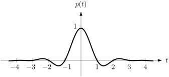
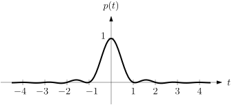
For more details, see BTD01.
Notes
- For $\alpha = 0$ it reduces to the sinc pulse.
Parameters:
-
rolloff(float) –The roll-off factor $\alpha$ of the pulse. Must satisfy $0 \leq \alpha \leq 1$. The default value is
1.0.
waveform()
The waveform $p(t)$ of the pulse.
For the Beaulieu pulse, it is given by $$ p(t) = \sinc(t) \frac{4 \beta \pi t \sin(\pi \alpha t) + 2 \beta^2 \cos(\pi \alpha t) - \beta^2}{(2 \pi t)^2 + \beta^2}. $$
Examples:
>>> pulse = komm.BeaulieuPulse(rolloff=0.25)
>>> pulse.waveform(
...     [-1.0, -0.75, -0.5, -0.25, 0.0, 0.25, 0.5, 0.75, 1.0],
... ).round(3)
array([0.   , 0.28 , 0.618, 0.894, 1.   , 0.894, 0.618, 0.28 , 0.   ])
spectrum()
The spectrum $\hat{p}(f)$ of the pulse.
Examples:
>>> pulse = komm.BeaulieuPulse(rolloff=0.25)
>>> np.abs(pulse.spectrum(
...     [-1.0, -0.75, -0.5, -0.25, 0.0, 0.25, 0.5, 0.75, 1.0],
... ))
array([0. , 0. , 0.5, 1. , 1. , 1. , 0.5, 0. , 0. ])
energy()
The energy $E$ of the pulse.
For the Beaulieu pulse, it is given by $$ E = 1 - \frac{\alpha}{4 \ln 2}. $$
Examples:
>>> pulse = komm.BeaulieuPulse(rolloff=0.25)
>>> pulse.energy()
0.9098315599444398
autocorrelation()
The autocorrelation function $R(\tau)$ of the pulse.
For the Beaulieu pulse, it is given by $$ \begin{aligned} R(\tau) = \sinc(\tau) ( 2 \cos(\pi \alpha \tau) - 1 ) & + \frac{4 \beta ( \cos(2 \pi f_1 \tau) + \cos(2 \pi f_2 \tau) ) + 4 \pi \tau ( \sin(2 \pi f_2 \tau) - \sin(2 \pi f_1 \tau) ) - 2 \beta \cos(\pi \tau)}{4 \beta^2 + (2 \pi \tau)^2} \\[1ex] & - \frac{4 \beta \cos(2 \pi f_2 \tau) + 8 \pi \tau \sin(2 \pi f_2 \tau) - 2 \beta \cos(\pi \tau) - 4 \pi \tau \sin(\pi \tau)}{\beta^2 + (2 \pi \tau)^2}. \end{aligned} $$
Examples:
>>> pulse = komm.BeaulieuPulse(rolloff=0.25)
>>> pulse.autocorrelation(
...     [-1.0, -0.75, -0.5, -0.25, 0.0, 0.25, 0.5, 0.75, 1.0],
... ).round(3)
array([0.084, 0.341, 0.618, 0.83 , 0.91 , 0.83 , 0.618, 0.341, 0.084])
energy_spectral_density()
The energy spectral density $S(f)$ of the pulse.
For the Beaulieu pulse, it is given by $$ S(f) = \begin{cases} 1, & |f| \leq f_1, \\[1ex] \mathrm{e}^{-2 \beta (|f| - f_1)}, & f_1 \leq |f| \leq 1/2, \\[1ex] ( 1 - \mathrm{e}^{-\beta (f_2 - |f|)} )^2, & 1/2 \leq |f| \leq f_2, \\[1ex] 0, & \text{otherwise}. \end{cases} $$
Examples:
>>> pulse = komm.BeaulieuPulse(rolloff=0.25)
>>> pulse.energy_spectral_density(
...     [-1.0, -0.75, -0.5, -0.25, 0.0, 0.25, 0.5, 0.75, 1.0],
... )
array([0.  , 0.  , 0.25, 1.  , 1.  , 1.  , 0.25, 0.  , 0.  ])
support tuple[float, float]
cached
property
The support of the pulse waveform $p(t)$, defined as the interval $[a, b]$ where $p(t)$ is non-zero.
For the Beaulieu pulse, the support is given by $(-\infty, \infty)$.
Examples:
>>> pulse = komm.BeaulieuPulse(rolloff=0.25)
>>> pulse.support
(-inf, inf)
taps()
Returns the FIR taps of the pulse.
Parameters:
-
samples_per_symbol(int) –The number of samples per symbol.
-
span(tuple[int, int] | None) –The time span to consider for the taps. This parameter is optional for pulses with finite support (defaults to $[0, 1]$), but required for pulses with infinite support.
Examples:
>>> pulse = komm.BeaulieuPulse(rolloff=0.25)
>>> pulse.taps(samples_per_symbol=4, span=(-1, 1)).round(3)
array([0.   , 0.28 , 0.618, 0.894, 1.   , 0.894, 0.618, 0.28 , 0.   ])
>>> pulse.taps(samples_per_symbol=4, span=(-16, 16)).shape
(129,)
root()
Returns the square-root version of the pulse, defined as the pulse whose spectrum is given by the square root of the spectrum of the original pulse. This method is only implemented for Nyquist pulses.
For the Beaulieu pulse, the waveform of the square-root version does not have a closed-form expression; it is computed here by numerical integration of the square root of the spectrum.
Examples:
>>> pulse = komm.BeaulieuPulse(rolloff=0.25).root()
>>> pulse.waveform(
...     [-1.0, -0.75, -0.5, -0.25, 0.0, 0.25, 0.5, 0.75, 1.0],
... ).round(3)
array([-0.08 ,  0.215,  0.611,  0.953,  1.087,  0.953,  0.611,  0.215,
       -0.08 ])
>>> np.abs(pulse.spectrum(
...     [-1.0, -0.75, -0.5, -0.25, 0.0, 0.25, 0.5, 0.75, 1.0],
... )).round(3)
array([0.   , 0.   , 0.707, 1.   , 1.   , 1.   , 0.707, 0.   , 0.   ])